pandas高阶应用

1、时间序列相关操作

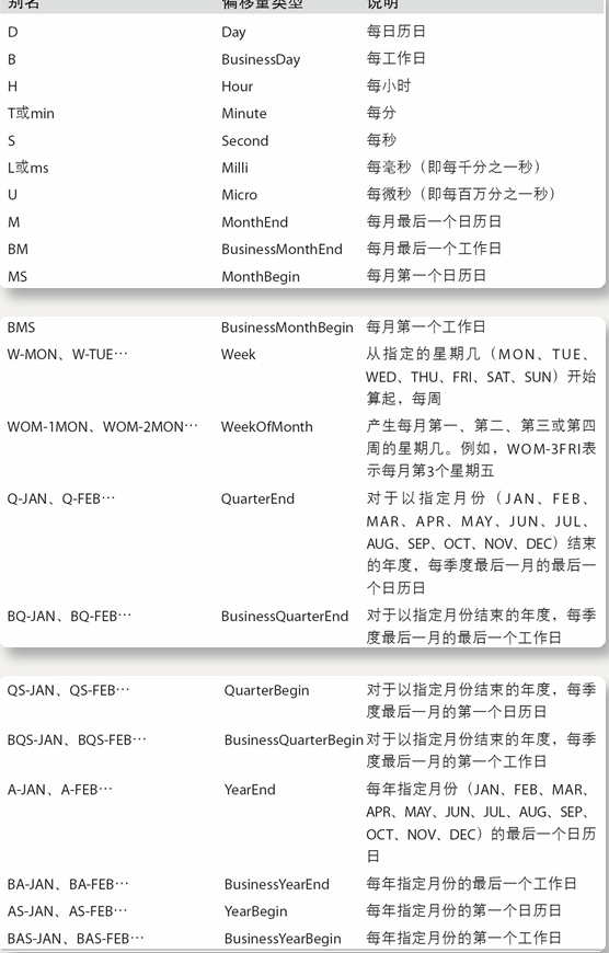
pd的date_range中的基本时间序列频率

2、三种透视图操作方法

import pandas as pd import numpy as np  v = [1, 2, 3, 3, 3] a = pd.DataFrame({'v': v}) d = [2 , 4, 4, 5, 4] a['d'] = d c = ['c' , 'h', 'd', 'e',  'c'] a['c'] = c a.head() ####a的数据状况为： 	v	d	c 0	1	2	c 1	2	4	h 2	3	4	d 3	3	5	e 4	3	4	c  # df用两个列进行分组groupby a.groupby(['v','d'])['c'].count() ### 分组结果为： v  d 1  2    1 2  4    1 3  4    2    5    1 Name: c, dtype: int64

将上步得到的数据行列转换：v列的值做index, d列的值做columns，将数据对应填入

以下为三种操作方法

2.1 crosstab

cpd = pd.crosstab(a['v'], a['d'], a['c'], aggfunc='count') cpd ## 结果为: d	2	4	5 v			 1	1.0	NaN	NaN 2	NaN	1.0	NaN 3	NaN	2.0	1.0 # 将上步所得结果空值填充为0 cpb.fillna(0,inplace=True)

2.2 pivot_tabel

a.groupby(['v', 'd'], as_index=False)['c'].count().pivot_table(     index=['v'],     columns=['d'],     values='c',     aggfunc='count').fillna(0) ## 结果为： d	2	4	5 v			 1	1.0	0.0	0.0 2	0.0	1.0	0.0 3	0.0	1.0	1.0

2.3 pivot

a.groupby(['v', 'd'], as_index=False)['c'].count() ## 结果为： 	v	d	c 0	1	2	1 1	2	4	1 2	3	4	2 3	3	5	1  a.groupby(['v', 'd'], as_index=False)['c'].count().pivot("v","d","c").fillna(0) ### 结果为：  d	2	4	5 v			 1	1.0	0.0	0.0 2	0.0	1.0	0.0 3	0.0	2.0	1.0

3、groupby后接各种便利操作

3.1 groupby本体

for ind,data in a.groupby(['v','d']):     print(ind,data)

3.2 groupby--agg

a.groupby(['v','d']).agg({"c":["count"]})  # 哪些列所需的函数操作只需要列为key, 函数作为value，或value list # 结果为： 		c count v	d	 1	2	1 2	4	1 3	4	2 5	1  # 常用的函数有：count,min,max,median,mean,sum,cumsum

3.3 groupby--transform

transform可使groupby的结果去索引化一一填充，作用类似a.groupby(['v', 'd'], as_index=False)['c'].count()

a.groupby(['v','d'])['c'].transform('count') ## 结果为: 0    1 1    1 2    2 3    1 4    2 Name: c, dtype: int64

4、apply

def func(x):     if x=="c":         x = 3     elif x=="d":         x = 4     elif x=="e":         x = 5     else:         x = 6     return x  a['c'].apply(func)  ## 结果为： 0    3 1    6 2    4 3    5 4    3  a['c'].apply(lambda x: 1 if x=="c" else 0)

5、多个sheet写入excel

pd.ExcelWriter(path) as fp:     df1.to_excel(fp,sheet_name="")     df2.to_excel(fp,sheet_name="")     df3.to_excel(fp,sheet_name="")

6、大数据加速处理Tips

6.1 分块读取

def get_df(file):     mylist = list()     for chunk in pd.read_csv(file,sep=',',chunksize=1000000):         mylist.append(chunk)     temp_df = pd.concat(mylist,axis=0)     del mylist     return temp_df

6.2 swifter--针对apply的加速包

# Swifter可以检查你的函数是否可以向量化，如果可以，就使用向量化计算 # 直接在apply在前面加上swifter就行 df.swifter.apply()

6.3 category

Pandas中有一种特殊的数据类型叫做category。它表示的是一个类别，一般用在统计分类中，比如性别，血型，分类，级别等等。

1. Categories是从数据中推断出来的。
2. Categories是没有大小顺序的。

会比原始数据类型占用的内存少。

但是category数据类型后续操作不方便，比如填充空值就会报错，可将其转化成对应的code

.astype('category').cat.codes---->直接将series分类后映射成数值。

6.4 glob--读取批量数据

glob包，这个包将一次处理多个csv文件。可以使用data/*. CSV模式来获取data文件夹中的所有csv文件。

pandas没有本地的glob支持，因此我们需要循环读取文件。

import glob all_files = glob.glob('data/*.csv') dfs = [] for fname in all_files:     dfs.append(pd.read_csv(fname, parse_dates=['Date'])) df = pd.concat(dfs, axis=0) dfsum = df.groupby(df['Date'].dt.year).sum() 

6.5 Vaex

1. Vaex 是一个开源的DataFrame库(类似于Pandas)，对和你硬盘空间一样大小的表格数据集，它可以有效进行可视化、探索、分析甚至进行实践机器学习。
2. Vaex 采用内存映射、高效的核外算法和延迟计算等概念。

1. Vaex 要求将CSV转换为HDF5格式，才能看到Vaex的优点。

HDF5是一种全新的分层数据格式产品，由数据格式规范和支持库实现组成。 HDF5旨在解决较旧的HDF产品的一些限制，满足现代系统和应用需求。 HDF5文件以分层结构组织，其中包含两个主要结构：组和数据集。 HDF5 group：分组结构包含零个或多个组或数据集的实例，以及支持元数据(metadata)。 HDF5 dataset：数据元素的多维数组，以及支持元数据。 但HDF5文件会比较大

import glob import vaex  # csv_files = glob.glob('csv_files/*.csv') csv_files = glob.glob('train.csv') for i, csv_file in enumerate(csv_files, 1):     for j, dv in enumerate(vaex.from_csv(csv_file, convert=True, chunk_size=5_000_000), 1):         print('Exporting %d %s to hdf5 part %d' % (i, csv_file, j))         dv.export_hdf5(f'hdf5_files/analysis_{i:02}_{j:02}.hdf5') dv = vaex.open('hdf5_files/*.hdf5') ### Vaex实际上并没有读取文件，因为延迟加载。### quantile = dv.percentile_approx('col1', 10) dv['col1_plus_col2'] = dv.col1 + dv.col2 dv['col1_binary'] = dv.col1> dv.percentile_approx（'col1'，10）